Series Resonant Converter (SRC)
A bridge inverter drives a series Lr–Cr tank in series with the load, so the tank behaves like a frequency-controlled valve. Sweep the switching frequency near resonance and the output follows — with soft switching, low EMI and near-sinusoidal currents. This is the simplest member of the resonant-converter family and the gateway to LLC.
- Introduction — switching softly, not squarely
- What is a Series Resonant Converter?
- Block Diagram
- Circuit Diagram & Construction
- Principle of Operation
- Modes of Operation (six switched states)
- Waveforms Explained in Detail
- Resonance, ZVS & ZCS — the three regions
- Voltage Gain & Frequency Control
- Key Formulas
- Worked Example
- Advantages & Disadvantages
- Applications
- Frequently Asked Questions – FAQs
- Related Topics
Introduction — switching softly, not squarely
Every hard-switched converter on this site — buck, boost, forward, the bridges — shares one problem: the switch turns on and off while it is carrying current and blocking voltage at the same instant. That overlap is switching loss, and it grows with frequency. It is the wall you hit when you try to shrink the magnetics by switching faster.
A resonant converter ducks around that wall. Instead of feeding the transformer a hard square wave, it feeds a square wave into an L–C resonant tank. The tank rings, so the current handed to the switches is a smooth near-sinusoid that naturally passes through zero. Time the switching to those zero crossings and the switch changes state while its current or voltage is (almost) zero — soft switching. Losses fall, EMI falls, and the converter can run at hundreds of kilohertz with a small, cool transformer.
The series resonant converter (SRC) is the simplest of the family: the tank inductor Lr and tank capacitor Cr sit in series with the load. That single choice explains everything the SRC does well and badly. This page builds it from the ground up — the circuit, the six switched modes, the waveforms, why it is run above resonance, the frequency-controlled gain curve, and the one weakness (light-load regulation) that led engineers to the LLC converter.
What is a Series Resonant Converter?
A series resonant converter is an isolated DC-DC converter in which a switching bridge drives a series Lr–Cr resonant tank that sits in the path between the source and the load. Output voltage is regulated by changing the switching frequency, not the pulse width. It is built from these parts:
- A switching bridge (inverter). A full bridge (Q1–Q4) or a half bridge chops the DC input Vg into a square-wave voltage vs of ±Vg (or 0 to Vg for a half bridge).
- A series resonant tank: Lr then Cr. This is the defining element. In series with the load, the tank forms a frequency-dependent divider — it passes energy easily at its resonant frequency and blocks it away from resonance.
- An isolation transformer. Provides galvanic isolation and scales the voltage by its turns ratio n. The tank current flows through the primary.
- An output rectifier + filter. A diode bridge (or synchronous rectifier) turns the near-sinusoidal tank current into DC, smoothed by a filter capacitor Cf across the load R.
The tank is characterised by two numbers. Its resonant frequency fr = 1 / (2π√(LrCr)) is where it rings; its characteristic impedance Zo = √(Lr/Cr) sets how hard it pushes back. The ratio of Zo to the (reflected) load resistance is the quality factor Q, which decides how sharply the output responds to frequency.
Block Diagram
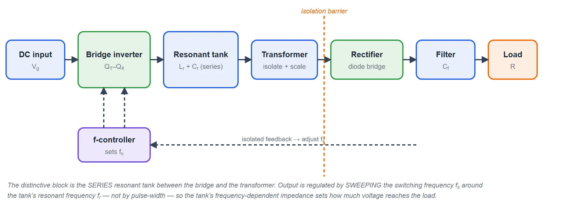
Read it left to right: the DC input is chopped by the bridge inverter into a square wave, filtered by the series resonant tank into a near-sinusoid, passed through the transformer, rectified and smoothed for the load. The control loop is what marks this as a resonant converter — feedback does not adjust a duty cycle; it adjusts the switching frequency, sliding the operating point along the tank’s gain curve.
Circuit Diagram & Construction
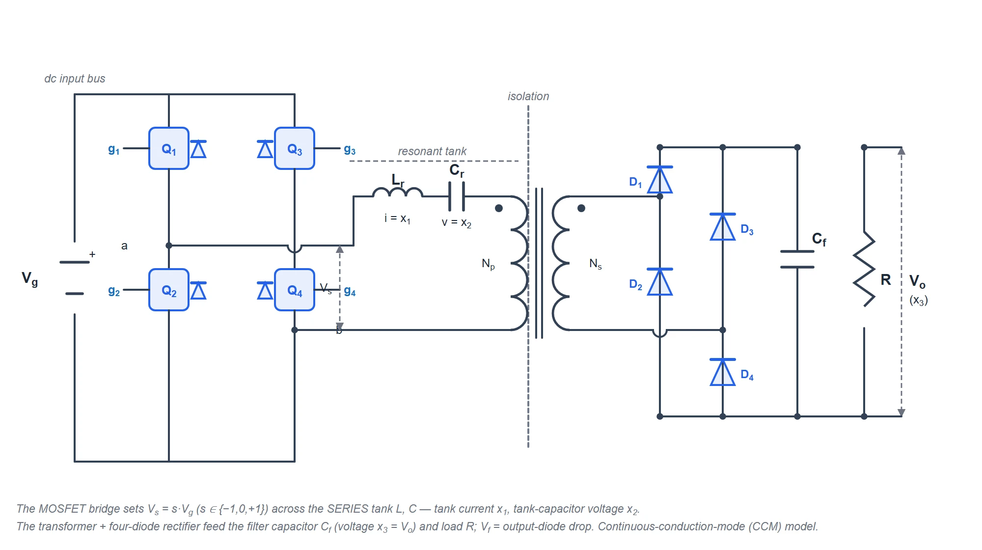
This is the power stage of the series resonant converter. What matters is not just the parts, but the three state variables the whole model is built on — so read the circuit in terms of them:
| x1 — tank inductor current | The current in the series resonant inductor L. It is the main resonating variable, and (as the next section shows) its sign decides which output diodes conduct. |
|---|---|
| x2 — tank capacitor voltage | The voltage across the series resonant capacitor C. The tank current x1 charges and discharges it every cycle. |
| x3 — filter capacitor voltage | The voltage across the output filter capacitor Cf — i.e. the output voltage delivered to the load R. |
| Vs — MOSFET-bridge output | The voltage the switching bridge applies to the tank. The switches set it to +Vg, 0 or −Vg; it is varied by frequency (and, in some designs, symmetrical-duty) control. |
Reading the power path from the input: a dc source Vg feeds a MOSFET bridge whose output Vs is a switched voltage; that drives the series resonant tank (inductor L and capacitor C in series); the tank current x1 passes through the transformer to the output diode rectifier, whose forward drop is written Vf; and the rectified current feeds the filter capacitor Cf and the load R.
Taking the converter to run in continuous conduction mode (CCM), the whole circuit can be written as a single nonlinear state-space model:
L · dx1/dt = s·Vg − x2 − rLoss·x1 − sgn(x1)·(x3 + 2Vf)C · dx2/dt = x1
Cf · dx3/dt = |x1| − x3/R
Each line is one physical law of the circuit above — worth reading term by term:
- Inductor equation. The tank current x1 is pushed by the bridge voltage s·Vg, opposed by the tank-capacitor voltage x2, by the loss drop rLoss·x1 (rLoss is the inductor resistance plus the capacitor’s series resistance), and by the reflected output term sgn(x1)·(x3+2Vf) — the output voltage plus two diode drops, with a polarity that follows the direction of the current.
- Tank-capacitor equation. C·dx2/dt = x1: the resonant capacitor simply integrates the tank current.
- Output equation. Cf·dx3/dt = |x1| − x3/R: the filter capacitor is charged by the rectified tank current |x1| and discharged by the load current x3/R.
- The logic input s. s ∈ {−1, 0, +1} is the logic input: it represents the state of the input switches and so fixes the bridge output Vs = s·Vg — +Vg, zero, or −Vg.
Principle of Operation
Think of the tank as a frequency-selective filter standing between the square-wave bridge and the load. A square wave is really its fundamental sine plus a stack of harmonics. A series Lr–Cr tank has its lowest impedance right at resonance, so it lets the fundamental through and heavily attenuates the harmonics. What reaches the transformer and load is therefore an almost pure sine wave at the switching frequency — this is the basis of the standard “first-harmonic approximation” used to analyse the SRC.
Now the key idea — how the frequency sets the output:
- At resonance (fs = fr), Lr and Cr cancel: the tank is a plain wire (just its small resistance). Almost the entire fundamental reaches the load, so the gain is at its maximum, M = 1. The current is exactly in phase with the square wave.
- Away from resonance (either side), the tank’s net reactance grows, dropping more of the voltage across Lr–Cr and less across the load. The gain falls. So moving the switching frequency away from fr turns the output down.
- The converter is normally operated above resonance (fs > fr). There the tank looks inductive, the current lags the voltage, and the switches get zero-voltage switching — the low-loss, low-EMI sweet spot for MOSFET bridges.
Because the tank passes only near-resonant energy, an SRC is a step-down converter: the best it can do is deliver the full fundamental at resonance (M = 1). It cannot boost. To raise or lower the output within that ceiling, the controller simply slews the frequency up (less output) or down toward fr (more output).
Modes of Operation (six switched states)
The cleanest way to describe the modes is to treat the converter as a switched system made of affine subsystems. The reason is simple: because the model above contains the two direction-dependent terms sgn(x1) and |x1|, the single nonlinear model splits into a set of ordinary linear pieces — one for every combination of the tank-current sign and the switch state. Counting them gives exactly six modes, shown as the six sub-circuits in the figure below. Each one is fixed by just two things:
- the sign of the tank current x1 (x1 > 0 or x1 < 0), which sets the sign of the reflected output term ±(x3+2Vf) and of the charging term ±x1 in the output equation; and
- the logic input s ∈ {+1, 0, −1}, which fixes the bridge voltage Vs = s·Vg. Here s = 0 is the dead-time state in the switching between the two switches.
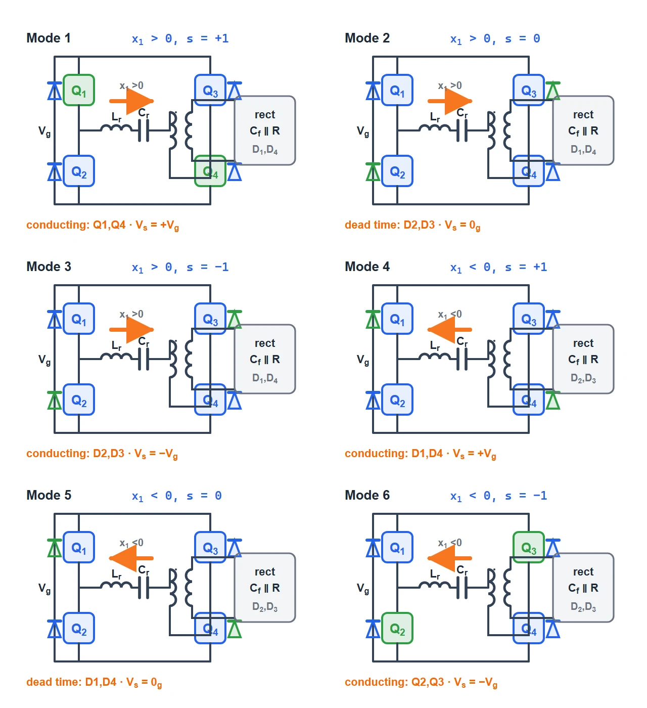
Writing the model out for each of the six conditions gives six affine (linear-plus-constant) systems. Only two things change from row to row — the s·Vg term (set by s) and the sign of the reflected output (x3+2Vf) and of the charging term (set by the sign of x1) — while the tank- capacitor equation C·dx2/dt = x1 is the same throughout:
| Mode | Condition | Vs | L·dx1/dt = | Cf·dx3/dt = |
|---|---|---|---|---|
| 1 | x1 > 0, s = +1 | +Vg | +Vg − x2 − rLossx1 − (x3+2Vf) | +x1 − x3/R |
| 2 | x1 > 0, s = 0 (dead time) | 0 | −x2 − rLossx1 − (x3+2Vf) | +x1 − x3/R |
| 3 | x1 > 0, s = −1 | −Vg | −Vg − x2 − rLossx1 − (x3+2Vf) | +x1 − x3/R |
| 4 | x1 < 0, s = +1 | +Vg | +Vg − x2 − rLossx1 + (x3+2Vf) | −x1 − x3/R |
| 5 | x1 < 0, s = 0 (dead time) | 0 | −x2 − rLossx1 + (x3+2Vf) | −x1 − x3/R |
| 6 | x1 < 0, s = −1 | −Vg | −Vg − x2 − rLossx1 + (x3+2Vf) | −x1 − x3/R |
Reading the table by the two halves of the switching cycle:
- Modes 1–3 (x1 > 0). The tank current is positive, so the reflected output term is −(x3+2Vf) and the filter capacitor is charged by +x1 (one output-diode pair conducts). Within this half the logic input steps the bridge through Vs = +Vg (mode 1), the dead-time state Vs = 0 (mode 2), and Vs = −Vg (mode 3).
- Modes 4–6 (x1 < 0). The current has reversed, so the other output-diode pair conducts: the reflected term flips to +(x3+2Vf) and the capacitor is charged by −x1 (= |x1|). Again s runs the bridge through +Vg, 0 and −Vg (modes 4, 5, 6).
Waveforms Explained in Detail
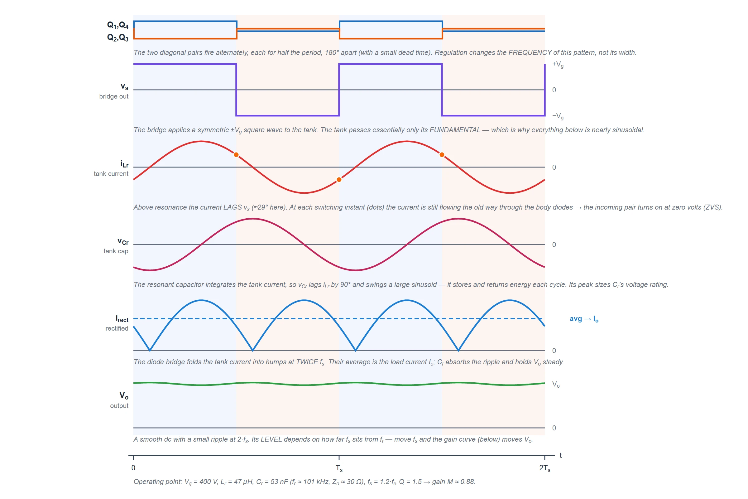
Read the traces together and the converter’s whole behaviour is in one picture:
- Gates. The two diagonal pairs fire alternately, each for about half the period, 180° apart, with a small dead time. Crucially, the controller regulates by changing the frequency of this pattern, not its width.
- Bridge voltage vs. A clean bipolar ±Vg square wave — the raw drive the tank has to filter.
- Tank current iLr. A near-sinusoid, because the tank passes essentially only the fundamental. Above resonance it lags vs (about 29° here). Look at each switching instant (marked): the current is still flowing the “old” way through the body diodes, so the incoming switches turn on at zero volts.
- Tank-capacitor voltage vCr. Cr integrates the current, so vCr lags iLr by 90° and swings a large sinusoid. It stores and returns energy every cycle; its peak sets the voltage rating of Cr and can exceed Vg.
- Rectified output current. The diode bridge folds iLr into a train of sine humps at twice the switching frequency. Their average is the load current Io.
- Output voltage Vo. Nearly flat, with only a small ripple at 2·fs that Cf smooths. Its level is set by how far fs sits from fr.
These are the fundamental (quasi-sinusoidal) waveforms — the standard way to picture an SRC. In a real converter the current is a slightly distorted sine, but the phase relationships and the soft-switching story are exactly as drawn.
Resonance, ZVS & ZCS — the three regions
Whether the SRC switches softly — and how — depends entirely on which side of resonance you operate. The tank current’s phase relative to the bridge voltage tells the whole story:
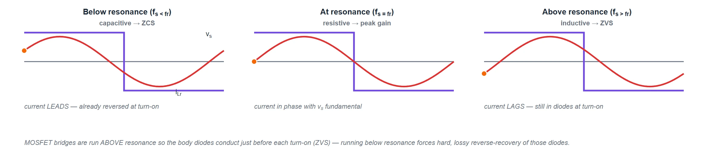
- Below resonance (fs < fr) — capacitive, ZCS. The net tank reactance is capacitive, so the current leads the voltage. Switches turn off near a current zero (zero-current switching). The catch: at turn-on the MOSFET body diode is forced to recover hard, which is lossy and noisy — so this region is generally avoided with MOSFETs (it can suit thyristor or IGBT designs).
- At resonance (fs = fr) — maximum gain. The tank is purely resistive, current and voltage are in phase, and the output is at its ceiling, M = 1.
- Above resonance (fs > fr) — inductive, ZVS. The current lags. During each dead time the tank current charges/discharges the switch capacitances and forces the incoming body diode to conduct, so the switch turns on at zero voltage. This is the region almost every MOSFET-based SRC (and LLC) is designed to live in.
Voltage Gain & Frequency Control
Using the first-harmonic approximation, the tank plus reflected load behaves like a series R–L–C driven by the fundamental of the square wave. That gives the SRC’s signature gain curve:
M(fn) = 1 / √( 1 + Q² · (fn − 1/fn)² ) where fn = fs/fr, Q = Zo/Rac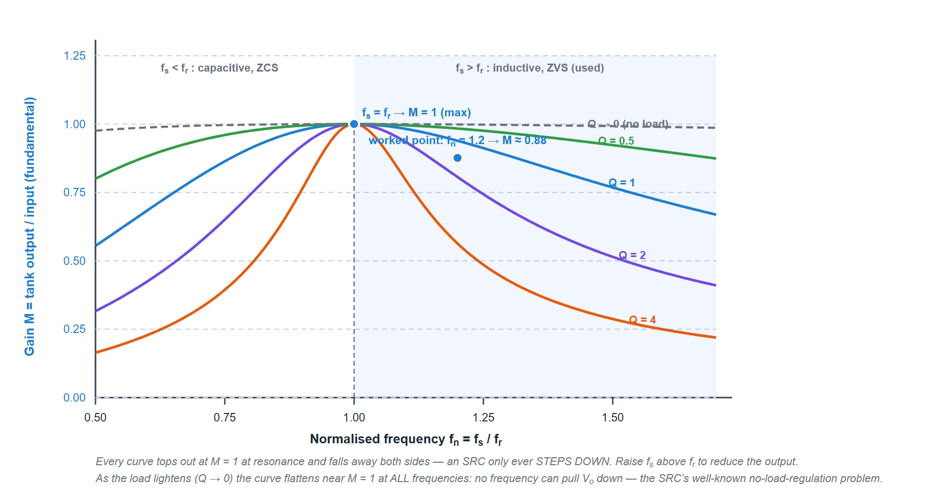
Three things to read off this curve, each a design consequence:
- It is always a step-down. Every curve tops out at M = 1 at resonance. An SRC cannot make its output larger than the input reflected through the turns ratio — it can only reduce it. To raise the output toward the ceiling, move fs down toward fr; to lower it, move fs up.
- Load changes the curve. Higher Q (lighter load impedance / higher load current) sharpens the peak; lower Q (heavy load) flattens it. A fixed frequency therefore gives different gains at different loads, so the controller must retune fs as the load moves.
- The no-load problem. As the load falls to zero, Q → 0 and the curve becomes almost flat at M ≈ 1 for every frequency. No frequency can pull the output down — to regulate a no-load SRC you would need an infinitely high frequency. This single limitation is the reason the LLC converter (which adds a parallel magnetising inductance to keep control at light load) largely replaced the plain SRC in modern supplies.
Key Formulas
| Resonant frequency | fr = 1 / (2π√(LrCr)) |
|---|---|
| Characteristic (surge) impedance | Zo = √(Lr/Cr) = ωrLr = 1/(ωrCr) |
| Loaded quality factor | Q = Zo / Rac |
| AC-equivalent load (full-bridge rectifier, cap filter) | Rac = (8/π²) · n² · R |
| Normalised frequency | fn = fs / fr |
| Fundamental voltage gain (tank) | M = 1 / √(1 + Q²(fn − 1/fn)²) |
| Output voltage (approx.) | Vo ≈ n · M · Vg (full bridge); ½ that for a half bridge |
| Peak gain / operating limit | Mmax = 1 at fn = 1; run at fn > 1 for ZVS |
Rac is the trick that makes the linear gain formula work: the diode rectifier plus its constant-voltage load do not look like a plain resistor to the tank, but to the fundamental they behave like an equivalent resistance Rac = (8/π²)·n²·R. Feeding that into a textbook series-RLC divider gives the gain curve above.
Worked Example
One consistent tank, used by every figure on this page. Follow the numbers and the curve checks out.
| Given | Vg = 400 V, Lr = 47 µH, Cr = 53 nF, full bridge |
|---|---|
| Resonant frequency fr = 1/(2π√(LrCr)) | 1 / (2π√(47µ × 53n)) ≈ 101 kHz |
| Characteristic impedance Zo = √(Lr/Cr) | √(47µ / 53n) ≈ 30 Ω |
| Operating frequency fs = 1.2·fr | ≈ 121 kHz (above resonance → ZVS) |
| Chosen load factor Q = Zo/Rac | 1.5 |
| Tank phase lag φ = atan(Q(fn−1/fn)) | atan(1.5 × (1.2 − 0.833)) ≈ 29° (current lags → inductive) |
| Voltage gain M = 1/√(1+Q²(fn−1/fn)²) | 1/√(1 + 1.5²×0.367²) ≈ 0.88 |
| To raise the output | lower fs toward fr (M → 1); to lower it, raise fs |
At fn = 1.2 the tank passes about 88 % of the fundamental to the (reflected) load, the current lags by ~29° so the bridge switches at zero voltage, and if the load lightens the controller must push fs higher to hold Vo — until, near no load, it simply runs out of room. Slide fs down toward 101 kHz and the gain climbs toward 1; that is the entire control law.
Advantages & Disadvantages
Advantages
- Soft switching. Run above resonance, the bridge turns on at zero voltage — low switching loss and high efficiency, especially at high frequency.
- Low EMI. The tank current is a near-sinusoid, not a hard-edged square, so high-frequency noise is far lower than in a hard-switched converter.
- Small, cool magnetics. Soft switching allows very high frequency, which shrinks the transformer; Lr can even be the transformer’s leakage.
- Inherent DC blocking. The series capacitor Cr stops any DC reaching the transformer, so the core can’t walk into saturation — no flux-balancing circuit needed.
- Natural short-circuit tolerance. Above resonance the tank impedance limits the current; a shorted output is a manageable, not catastrophic, condition.
Disadvantages
- Step-down only. The gain never exceeds M = 1; the SRC cannot boost.
- Poor light-load / no-load regulation. As Q → 0 the gain flattens near 1, so the output can’t be pulled down at light load without impractically high frequency — the SRC’s defining weakness.
- Variable-frequency control complicates EMI filtering and magnetic design (the operating frequency is a moving target) and can demand a wide frequency range.
- Large circulating current. Energy sloshes in the tank each cycle (big vCr), adding conduction loss even at light load.
- Output ripple. With only a capacitor filter and pulsed diode current, output ripple current in Cf is high — the capacitor must be rated for it.
Applications
- High-voltage DC supplies (X-ray, electrostatic, laser, CRT) — the tank naturally handles the transformer’s large leakage and parasitic capacitance, and limits fault current.
- Induction heating and ultrasonic drives, where a resonant load is the point.
- Battery chargers and telecom rectifiers that run at a fairly constant load, where the no-load weakness doesn’t bite.
- The conceptual parent of the LLC converter — today’s dominant isolated DC-DC topology for PC, server and adapter supplies, which is a series resonant converter with an added parallel inductance to fix light-load regulation.
- Teaching and analysis — the SRC is the cleanest place to learn resonant conversion, ZVS/ZCS and frequency control before tackling LLC or LCC.
In short: the SRC is the foundation of soft-switched conversion. Where the load is steady it is used directly; where the load swings from full to zero, its close relative the LLC converter takes over — but LLC only makes sense once you understand the series resonant converter first.
Frequently Asked Questions – FAQs
Related Topics
- Full-Bridge Converter — the hard-switched bridge the SRC softens
- Half-Bridge Converter — a common SRC front end
- Forward Converter — the single-switch isolated buck
- Flyback Converter — the low-power isolated buck-boost
- MOSFET — the resonant-bridge switch and its body diode
- DC-DC Converters — Overview
- All Power Electronic Converters