Compensation Theorem
When one branch's resistance or impedance changes by ΔZ, you don't have to re-solve the whole circuit. The effect everywhere is exactly the response to a single compensating source Vc = −I·ΔZ placed in that branch, with all other sources switched off. Learn the statement, formula, derivation, sign convention, a full worked example and where it's used.
Complete Learning Path — Compensation Theorem
From the statement and formula, through a worked circuit and the compensation model, to the derivation, procedure, sign convention and applications
What is the Compensation Theorem?
The Compensation Theorem tells you how a network reacts when one branch changes. If a branch carrying current I has its impedance change by ΔZ, the resulting changes everywhere else are exactly what a single compensating source Vc = −I·ΔZ would produce — placed in that branch with all other independent sources turned off.
It is one of the classic network theorems, and it saves you from re-solving an entire circuit just to see the effect of tweaking one element — the essence of sensitivity analysis.
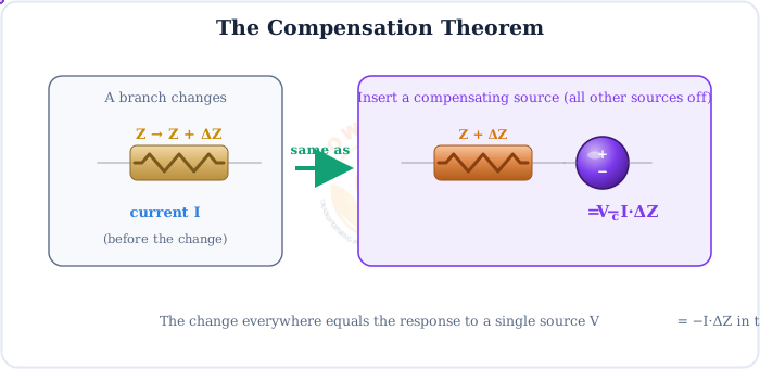
A change, not a replacement
The theorem models the effect of a change. That makes it a close cousin of the Substitution Theorem and a natural partner to Thévenin's theorem.
Statement & Formula
In a linear network, if a branch carrying current I has its impedance changed by ΔZ, the change in every current and voltage equals the response to a compensating EMF in that branch:
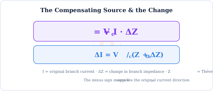
Vc = −I·ΔZ · ΔI = Vc / (Zth + ΔZ)
I = original branch current, ΔZ = change in branch impedance, Zth = Thévenin impedance seen by the branch
Why it helps
Instead of re-analysing the full circuit for the new element value, you solve one simple network driven by Vc alone — then add the change to the original answers.
A Worked Circuit
Start with a circuit whose branch current we know exactly. A 12 V source feeds a 2Ω resistor and a 4Ω branch in series.
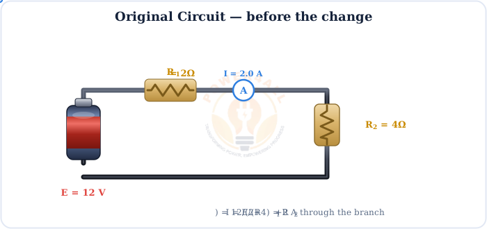
This original current, I = 2 A, is the number the compensating source will use. Note it down before touching the branch.
Now the Branch Changes
Suppose the 4Ω branch rises to 6Ω — a change of ΔR = +2Ω. The current will fall; the theorem lets us find by exactly how much.
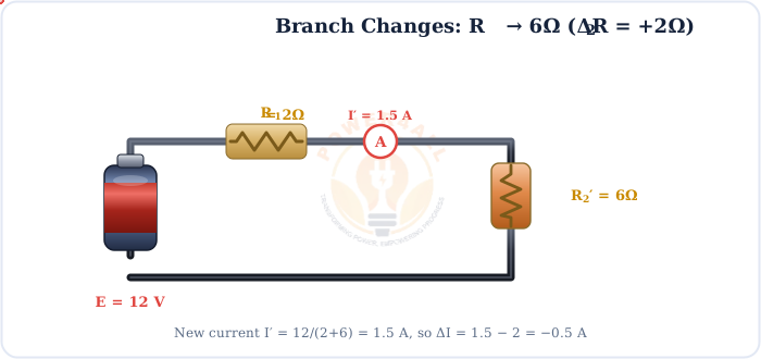
We already know the answer here because the circuit is tiny — but the Compensation Theorem gives the same ΔI in a way that scales to networks far too big to re-solve by hand.
The Compensation Model
Here's the trick: deactivate the source (short the 12 V battery), give the branch its new value 6Ω, and insert the compensating source Vc = −I·ΔR = −(2)(2) = −4 V. Solving this one loop gives ΔI directly.
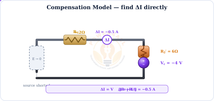
Deactivate means...
Replace independent voltage sources with a short circuit and independent current sources with an open circuit — the same rule you use in superposition and Thévenin.
Derivation
The result drops straight out of comparing the branch before and after the change.
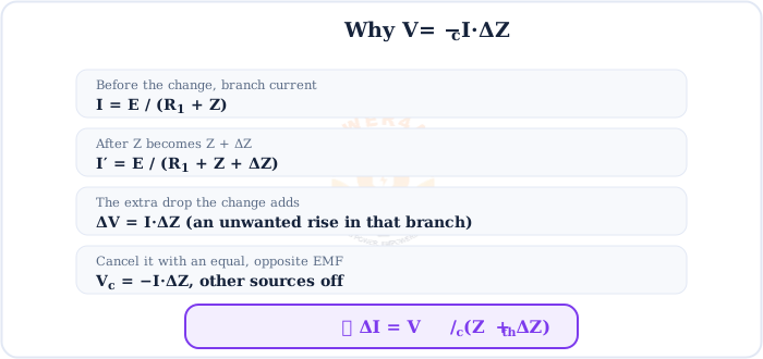
See the reasoning in full
1. Originally the branch impedance Z carries current I, dropping I·Z.
2. After the change the impedance is Z + ΔZ; at the (as-yet unknown) new current it drops (I+ΔI)(Z+ΔZ).
3. The extra voltage the change introduces, referred to the original current, is I·ΔZ. Everything else in the network is linear, so by superposition the change ΔI is the response to this extra voltage acting alone.
4. Modelling that extra voltage as a source that opposes the current gives Vc = −I·ΔZ, and with all real sources dead, ΔI = Vc/(Zth + ΔZ).
Worked Example
Putting the numbers together for our circuit — and checking against a direct solve.
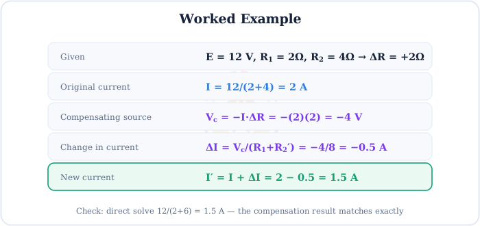
Step by step
Original current: I = 12/(2+4) = 2 A.
Compensating source: Vc = −I·ΔR = −(2)(2) = −4 V.
Change: ΔI = Vc/(R1+R2′) = −4/(2+6) = −0.5 A.
New current: I′ = 2 − 0.5 = 1.5 A (check: 12/(2+6) = 1.5 A). ✔
Step-by-Step Procedure
The same five steps work for any single-element change in a linear network.
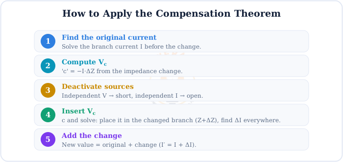
The Sign & Direction of Vc
The minus sign in Vc = −I·ΔZ is not decoration — it fixes the source's polarity.
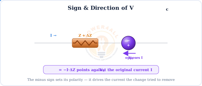
Get the polarity right and ΔI comes out with the correct sign automatically — here a negative ΔI, because increasing the resistance reduces the current.
Applications
The Compensation Theorem shines whenever one thing changes and you want the effect without redoing everything.

Sensitivity analysis
Quantify how one element's change ripples through every current and voltage.
Bridges & strain gauges
A tiny ΔR in a Wheatstone arm gives a small, easily-computed output change.
Small-signal / incremental
Model a small parameter shift around an operating point.
With Thévenin
Use Zth seen by the branch to get ΔI in a single division.
Key Terms at a Glance
The essential compensation-theorem vocabulary.
ΔZ (or ΔR)
The change in a branch's impedance.
Vc
Compensating source, −I·ΔZ.
ΔI
The resulting change in current.
Deactivate
V source → short, I source → open.
Zth
Thévenin impedance at the branch.
Original current
I before the change.
Frequently Asked Questions
Quick, expert answers to the questions people ask most about the Compensation Theorem.
What is the Compensation Theorem in simple words?
If one branch of a circuit changes its resistance or impedance by ΔZ, the effect on the rest of the circuit is the same as adding a small source Vc = −I·ΔZ in that branch, with all the real sources switched off.
What is the formula?
Vc = −I·ΔZ and ΔI = Vc/(Zth + ΔZ), where I is the original branch current, ΔZ the change, and Zth the Thévenin impedance seen by the branch.
Why is Vc negative?
The minus sign orients the compensating source to oppose the original current. It represents the extra drop I·ΔZ that the change introduces.
How do I apply it?
Find the original current I, compute Vc = −I·ΔZ, deactivate all independent sources, insert Vc in the changed branch and solve for ΔI, then add it to the originals.
When would I use it?
To find the effect of changing one element without re-solving the whole network — sensitivity analysis, Wheatstone bridges and strain gauges, and small-signal or incremental changes.
Does it work for AC circuits?
Yes. Use complex impedances: ΔZ and Vc = −I·ΔZ become phasor quantities, and the same procedure applies.
How is it different from the Substitution Theorem?
Substitution replaces a branch with an equivalent that has the same V and I. Compensation specifically models the effect of a change using a compensating source with other sources off.
What does it assume?
A linear network with a unique solution, so the change can be treated separately by superposition as the response to Vc acting alone.
Conclusion & Key Takeaways
The Compensation Theorem turns "what if this element changes?" into a single small calculation — the response to Vc = −I·ΔZ.
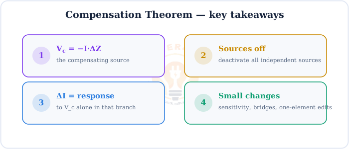
Vc = −I·ΔZ
The compensating source.
Sources off
Deactivate independent sources.
Solve for ΔI
Response to Vc alone.
Add it back
New value = old + change.
Opposes I
The minus sign sets polarity.
Great for changes
Sensitivity, bridges.